Four Tesla V100s, one vLLM engine, and 360 real ShareGPT conversations pushed through it. This post defines every metric before it reports one, shows the serving flags we actually ran and what each one costs, and ends where a benchmark should end — in a provisioning decision.

Why the usual dashboard cannot answer this

Open the monitoring page for almost any production service and you will find the same four panels: requests per second, error rate, response time, CPU and memory utilisation. Those panels have carried the industry for twenty years and they are not broken. They are answering a question a language model does not ask.

It is tempting to say that traditional monitoring failed for AI workloads. It did not. It was never designed for them. Request counts and endpoint latencies were built for services where a request is an indivisible unit of work: it arrives, it is handled, it departs, and the only interesting number is how long the whole thing took. CPU and memory mattered because CPU and memory were the contended resources. None of those assumptions were wrong — they were simply written before anyone was serving a model that streams its answer back one fragment at a time, on hardware whose contended resources are GPU compute and GPU memory bandwidth.

A language model request is not indivisible. It has internal structure, and the user experiences that structure directly. Someone waiting on a chat window feels two separate things — how long before anything appears, and how fast it flows once it starts. Averaging both into a single request duration discards exactly what they can feel. So the first move is not a better dashboard. It is changing the unit of measurement from the request to the token.

That is what the rest of this post does. It is the measurement we promised in how to read LLM inference numbers, run on our own hardware, with the numbers traced back to a recorded benchmark rather than a vendor slide.

The five numbers, and what each one actually means

Every figure in this post is one of five measurements. They are worth defining precisely, because each is quoted constantly and defined rarely, and because two of them are routinely confused with each other.

Metric	What it is	Unit	Who feels it
TTFT — time to first token	Request leaves the client → first content token comes back	ms	Anyone watching a cursor blink
TPOT — time per output token (= inter-token latency, ITL)	(end-to-end − TTFT) ÷ (output tokens − 1)	ms/token	Anyone reading the answer as it streams
Output tok/s	1000 ÷ TPOT — the same measurement, inverted	tokens/s	Same person, friendlier unit
E2E — end-to-end latency	Request start → stream complete	s	Anything waiting for the whole answer: agents, pipelines, API callers
Concurrency (C)	Requests in flight at one instant	count	The engine. Not the same as user count

Time to first token, properly

Whose clock is it? TTFT runs on the user’s clock, not the server’s. It starts when the request leaves the client and stops when the first content token comes back. Because the clock runs client-side, the measurement includes network transit, admission and queueing at the engine, tokenisation of the prompt, and the model’s first forward pass. Any measurement that starts the clock inside the server is measuring something narrower, and it will flatter you. A token is roughly three-quarters of a word, so in plain terms TTFT is the wait before the first word lands.

What is the unit? Seconds, conventionally reported in milliseconds. But a single TTFT figure is close to meaningless, because TTFT is a distribution. The engine exports it as a histogram — buckets counting how many requests landed in each latency band — and the honest way to summarise a histogram is by percentile, never by average. One long request drags a mean around; it cannot move a median.

When does it matter? TTFT dominates the felt experience of anything a person is waiting on — chat, assistants, interactive retrieval, autocomplete. It matters very little for offline and batch work, where nobody is watching a screen and only total tokens per hour count. Optimising TTFT for a nightly classification job is wasted effort.

Time per output token, and its inverse

Once the first token has arrived, TPOT is the average gap between every token after it — computed as (E2E − TTFT) ÷ (output tokens − 1). The minus one is not pedantry: the first token was already paid for by TTFT, so including it double-counts the prefill.

Output tokens per second is the same number turned upside down — 1000 ÷ TPOT — and it is the friendlier of the two because it maps onto a human reference point. Comfortable adult reading is somewhere near 6 tokens per second. Anything faster than that and the model is outrunning the reader, which is why the difference between 33 and 38 tokens per second is invisible to a person, while the difference between 33 and 4 is the difference between a product and a complaint.

One warning: per-stream tokens per second is not the same as the machine’s tokens per second. One user getting 38 tok/s and eight users each getting 33 tok/s are wildly different loads on the same box. We report both, and label which is which.

End-to-end latency

The total wall-clock time from request start to the end of the stream. E2E is roughly TTFT + (output tokens × TPOT), which means it is dominated by how much you asked the model to write, not by how fast the hardware starts. This is the metric that matters for agents and pipelines, where no human is reading along and the only question is when the complete answer is available for the next step.

Percentiles: p50, p95, p99

A percentile answers “how fast were the fastest N% of requests?”. p50 is the median — the typical user. p95 means ninety-five of every hundred requests were at least this fast, so it describes the slow tail most people will occasionally hit. p99 is the worst one in a hundred.

The reason to carry all three is that the gap between them is a measurement in its own right. When p50 and p99 sit on top of each other, the engine is idle and the work is deterministic. When they fan apart, requests are queueing behind one another — and the people who file support tickets are living on the p99 line, not the median. Provision on medians and you will ship something that tests beautifully and generates complaints.

Concurrency is not user count

Concurrency means requests in flight at the same instant. A team of fifty people using a chat assistant rarely puts more than a handful of requests in flight at once, because humans spend most of their time reading and typing. Sizing against headcount instead of observed in-flight requests is the single most common way to buy several times the GPUs you need.

One thing this post does not measure: whether the answers are any good. Latency and quality are separate instruments. Guardrails, hallucination detection, bias and fairness checks belong in the same operational picture, on their own dashboards. A system that is fast and wrong is not a system that works.

Why the numbers move: prefill and decode

Every result below follows from one fact: a request is served in two phases that behave nothing alike.

Prefill is the request-processing phase. The entire input prompt is read at once, the model builds its key–value cache for every prompt token in parallel, and the first output token is produced. Because the whole prompt is processed together, the work is a large matrix–matrix multiplication that saturates the GPU’s arithmetic units. Prefill is compute-bound, its cost scales with prompt length, and prefill is what TTFT measures.

Decode is everything after. The model emits one token, appends it to the context, and runs again — strictly sequential, one token at a time. Each step does very little arithmetic but must stream the model’s entire weight set out of GPU memory to produce that one token. Decode is memory-bandwidth-bound, its cost scales with output length, and decode is what TPOT measures.

That asymmetry predicts everything. Adding concurrent requests adds prefill work, which competes for the same arithmetic units, so TTFT climbs — sharply when the prompts are long. Decode reacts the opposite way: because it is bandwidth-limited rather than compute-limited, batching several sequences together lets the engine amortise a single weight read across all of them, so per-stream generation speed barely notices the extra company. Long input hurts time-to-start. Long output hurts total time. Concurrency hurts time-to-start far more than it hurts streaming speed. Hold those three sentences and the charts below will contain no surprises.

The hardware: four Tesla V100s on one node

NVIDIA Tesla V100-SXM2-16GB. Volta architecture, compute capability 7.0, 16 GB of HBM2 at roughly 900 GB/s, first-generation tensor cores delivering on the order of 125 TFLOPS of FP16 matrix throughput. In 2017 it was the fastest accelerator money could buy, and it is the card that made large-scale deep learning practical. All four sit in a single node — berry-gpu05 — on our berry-ai OpenShift cluster, connected by NVLink.

	V100-SXM2	A100-SXM 80GB	H100-SXM
Architecture	Volta (2017)	Ampere (2020)	Hopper (2022)
Compute capability	7.0	8.0	9.0
Memory	16 GB HBM2	80 GB HBM2e	80 GB HBM3
Memory bandwidth	~900 GB/s	~2,039 GB/s	~3,350 GB/s
bfloat16 / FP8	No / No	Yes / No	Yes / Yes
FlashAttention	Not supported	Yes	Yes

Two rows do most of the damage, and both are worth understanding before reading a single result.

Memory bandwidth, because decode is bandwidth-bound. Per-stream generation speed scales roughly with how fast weights can be pulled out of memory, and an H100 has close to four times the V100’s bandwidth. That is a hard ceiling on tokens per second per user which no amount of software tuning will lift. When you see 31–38 tok/s below, that is the number this row buys.

Compute capability 7.0, because much of the modern inference stack simply refuses to run below 8.0. FlashAttention needs Ampere or newer, so vLLM falls back to an older attention backend. The fast quantised-inference kernels need Ampere or newer, so 4-bit weights are off the table. vLLM’s V1 engine dropped pre-Ampere cards, so Volta stays on the older engine path. The hardware is not the only constraint here — the software ecosystem has moved on, and that is part of what you are buying, or not buying.

What the V100 still has: enough memory, in groups of four, for a 7B model at half precision with room for a healthy cache; wide availability; and a low price per card. For workloads that value total throughput over per-user speed, that remains genuinely economical — and it is a card that already exists, which is its own sustainability argument.

The model: RedHatAI Qwen2.5-7B-Instruct

Open-weight and instruction-tuned: 7.6 billion parameters across 28 transformer layers, a 3,584-dimension hidden state, 28 attention heads, and a natively supported context window of 32,768 tokens. We serve Red Hat’s validated build of it, which is what our RHOAI-based serving path expects — the weights are Qwen’s, the packaging and validation are Red Hat’s.

Three of its characteristics shape the measurements directly, so it is worth being explicit about them rather than treating the model as a black box.

Its size sets the memory floor. At fp16, 7.6 billion parameters occupy about 15.2 GB before a single token of conversation is stored. A V100 has 16 GB. That one comparison determines the entire deployment shape, and it is the reason the tensor-parallel flag in the next section is arithmetic rather than preference.

It uses grouped-query attention. Rather than 28 key–value heads to match its 28 attention heads, it has 4 — several attention heads share one set of keys and values. The KV cache, the per-token memory that lets the model attend to everything it has already seen, therefore costs roughly 56 KB per token instead of about seven times that. This is not a footnote. It is why cache memory never became the binding constraint at any concurrency we measured, and why the engine degraded in latency rather than failing under load.

7B is the useful middle. Coherent enough for chat, retrieval-augmented answering, summarisation and structured extraction; small enough to serve on hardware where a 70B model would not fit at any precision. The question this post asks — what does one engine on four old cards actually deliver — only makes sense at this size.

One caveat we would rather state than bury: Qwen2.5 was trained in bfloat16 and we serve it in float16. Both are 16-bit, but bfloat16 trades mantissa precision for a much wider exponent range. Casting down is standard practice and produces good output — it is still a deviation from the training format, and on this hardware it is not optional.

The serving configuration, flag by flag

The model is served through KServe on OpenShift AI. This is the ServingRuntime that was live on berry-gpu05 when the benchmark ran — reproduced rather than reconstructed:

apiVersion: serving.kserve.io/v1alpha1
kind: ServingRuntime
metadata:
  name: vllm-v100-tp4
spec:
  containers:
    - name: kserve-container
      image: vllm/vllm-openai:v0.8.5
      command: ["python", "-m", "vllm.entrypoints.openai.api_server"]
      args:
        - "--port=8080"
        - "--model=/mnt/models"
        - "--tensor-parallel-size=4"
        - "--dtype=half"
        - "--enforce-eager"
        - "--no-enable-prefix-caching"
        - "--max-model-len=8192"
        - "--gpu-memory-utilization=0.92"
      env:
        - name: HF_HUB_OFFLINE
          value: "1"
        - name: TRANSFORMERS_OFFLINE
          value: "1"
      resources:
        limits:
          cpu: "8"
          memory: 48Gi
          nvidia.com/gpu: "4"
        requests:
          cpu: "4"
          memory: 32Gi
          nvidia.com/gpu: "4"

Stripped of Kubernetes, that is the equivalent of:

vllm serve /mnt/models \
  --served-model-name redhataiqwen25-7b-instruct \
  --tensor-parallel-size 4 \
  --dtype half \
  --max-model-len 8192 \
  --gpu-memory-utilization 0.92 \
  --no-enable-prefix-caching \
  --enforce-eager

Every one of those flags moves a number in this post. Taking them in turn.

--tensor-parallel-size 4

Tensor parallelism splits each layer’s weight matrices across GPUs, so all four cards work on the same token simultaneously and combine their partial results. It is not the same as running four copies of the model — that would be data parallelism, and it would not help here at all.

Why 4 and not 1. Arithmetic, not preference. 15.2 GB of fp16 weights cannot sit on a 16 GB card and still leave room for a KV cache. TP=2 would fit — roughly 7.6 GB of weights per card — and TP=4 puts about 3.8 GB on each, freeing something like 11 GB per card for cache and activations.

What it buys. Splitting the weights divides the memory traffic each GPU must sustain per decode step by four, which is a real gain on a bandwidth-bound phase, and it leaves far more room for concurrent sequences.

What it costs. Every layer now ends in an all-reduce: the four GPUs must exchange and sum their partial results before the next layer can start. That synchronisation happens 28 times per token, on every token, for every request. You never get a clean 4× — you get most of the memory benefit minus a communication tax, and that tax is paid on the interconnect. It is also why a node with degraded GPU peer-to-peer underperforms in a way that looks nothing like a GPU problem, and why NCCL needs real shared memory to work with. Kubernetes gives a pod 64 MB of /dev/shm by default; that is nowhere near enough, and the failure mode is not an error message but a server that hangs silently on startup. It is the least obvious line in any of these manifests and the one most likely to cost you an afternoon.

One hard constraint: the tensor-parallel degree must evenly divide the model’s sharded dimensions. Qwen2.5-7B has 4 key–value heads, so TP=2 and TP=4 are both valid. TP=8 is not, on any hardware.

--dtype half

half is fp16. It is less a decision than the only survivor once you list the alternatives on Volta:

Option	Weights	Verdict on V100
float32	~30.5 GB	Doubles memory traffic on a bandwidth-bound phase, for no quality gain worth having.
bfloat16	~15.2 GB	The training format — but Volta has no native bfloat16 support.
half / fp16	~15.2 GB	Chosen. Native tensor-core support since Volta.
fp8	~7.6 GB	Hopper only.
4-bit AWQ / GPTQ	~4.5 GB	The fast kernels require compute capability ≥ 8.0.

On an Ampere or Hopper card that table reads completely differently, and that is a substantial part of why newer GPUs serve more users per euro. They can hold the same model in a third of the memory and spend everything they save on KV cache.

--max-model-len 8192

The model natively supports 32,768 tokens; we cap it at 8,192. At roughly 56 KB per token, a fully extended 8,192-token sequence occupies about 459 MB of KV cache; at 32,768 it would occupy about 1.8 GB each, and a handful of such conversations would consume the entire pool.

Capping context is how you convert an unbounded worst case into a predictable one. It guarantees the engine can admit a known number of sequences without preempting anyone, at the cost of refusing genuinely long documents. And because prefill time scales with prompt length, a context cap is indirectly a latency cap too — it puts a ceiling on how bad any single request’s TTFT can get.

--gpu-memory-utilization 0.92

The fraction of each card vLLM claims up front — about 14.7 GB of each 16 GB card — nearly all of which becomes KV cache once the weights are loaded. Higher values admit more concurrent sequences before the engine starts preempting; too high and an allocation spike triggers an out-of-memory error at exactly the wrong moment. At 0.92 there is roughly 1.3 GB of headroom per card, which held for every cell we ran.

It is worth checking that figure against the results. With weights sharded four ways, the cache pool is on the order of 43 GB across the node. At 56 KB per token that is roughly 800,000 cached tokens. Even the longest prompts in this benchmark, at eight in flight, occupied a small fraction of it. KV cache was never the binding constraint in these measurements — compute and bandwidth were. Worth knowing before concluding that a larger-memory card would have fixed the latency. It would not have.

--no-enable-prefix-caching

Prefix caching lets the engine reuse the KV cache for a prompt prefix it has already processed — hugely effective when many requests share a long system prompt, which is the normal shape of a RAG or agent deployment. We disabled it deliberately for the benchmark, because leaving it on would let cache hits flatter the TTFT numbers on repeated prompts and we would be publishing a cache-hit rate dressed up as hardware performance.

The consequence: the TTFT figures below are a cold-prefill floor. A production deployment with a shared system prompt and prefix caching enabled should do better than this on first-token latency, sometimes dramatically. We would rather understate.

--enforce-eager

This disables CUDA graph capture, so every forward pass is dispatched step by step instead of replayed as a pre-recorded graph. CUDA graphs remove per-step kernel launch overhead and are typically worth single-digit to low-double-digit percentages on decode, particularly at small batch sizes where launch overhead is a large fraction of the total work.

We run with it disabled because it stabilised first boot on Volta, and a server that starts reliably beats a server that is a few percent faster. The consequence for this post is the same as the flag above: the generation numbers are conservative, with known headroom deliberately left on the table.

Two things you will not find in that config and might expect to. There is no FlashAttention setting, because Volta cannot run it — vLLM selects an older attention backend on its own. And there is no V1-engine tuning, because vLLM’s V1 engine requires compute capability 8.0 or newer and falls back to the previous engine path here automatically. Neither is a choice we made; both are consequences of the card.

The workload: real conversations, in three shapes

A benchmark is only as honest as its prompts. Synthetic filler of a fixed length is excellent for isolating one variable and terrible for predicting real behaviour, because real traffic varies wildly in prompt length and that variance is precisely what stresses prefill.

So we drove this run from ShareGPT — the anon8231489123/ShareGPT_Vicuna_unfiltered dataset on Hugging Face, a corpus of real multi-turn conversations between people and assistants. It is the de-facto standard corpus for LLM serving benchmarks for exactly this reason: the prompt-length distribution is one that actually occurred. Sampling was seeded (seed=42) and the selected prompt set was hashed, so the run is reproducible rather than merely repeatable.

Those conversations were sorted into three buckets, because the prefill/decode split means a single average would hide the only distinction that matters:

Bucket	Shape	Stresses	Looks like
Long prompt → short answer	Big input, ~64 output tokens	Prefill	RAG, document Q&A, classification over retrieved context
Balanced chat	Moderate input, ~256 output tokens	Both	An ordinary assistant turn
Short prompt → long answer	Small input, ~512 output tokens	Decode	“Write me a…”, drafting, code generation

Each of the twelve cells — three buckets × four concurrency levels (1, 2, 4, 8) — ran 30 measured requests after 5 warmup requests, streaming against the OpenAI-compatible /v1/chat/completions endpoint. Warmup matters: the first request into a cold engine pays for CUDA context setup and memory allocation, and including it would poison the percentiles.

Critically, the client talked straight to the vLLM predictor — no gateway, no router, no proxy. These are engine-ceiling numbers. We measure the gateway hop separately further down, because conflating the two is how benchmarks become marketing.

Two honest notes on provenance. First, the raw per-request JSON lived on a Kubernetes Job emptyDir and was not copied off before the pod exited; the summary percentiles survived and are what we publish. Second, that summary did not record input token counts per bucket, so we describe prompt lengths relatively rather than inventing figures. Output lengths in the table above are derived: (E2E p95 − TTFT p95) × decode rate lands within a few percent of 64, 256 and 512 tokens in every one of the twelve cells, which is a strong consistency check on the data but is not the same as reading it from a log.

What the numbers say

First token: prompt length is the variable that matters

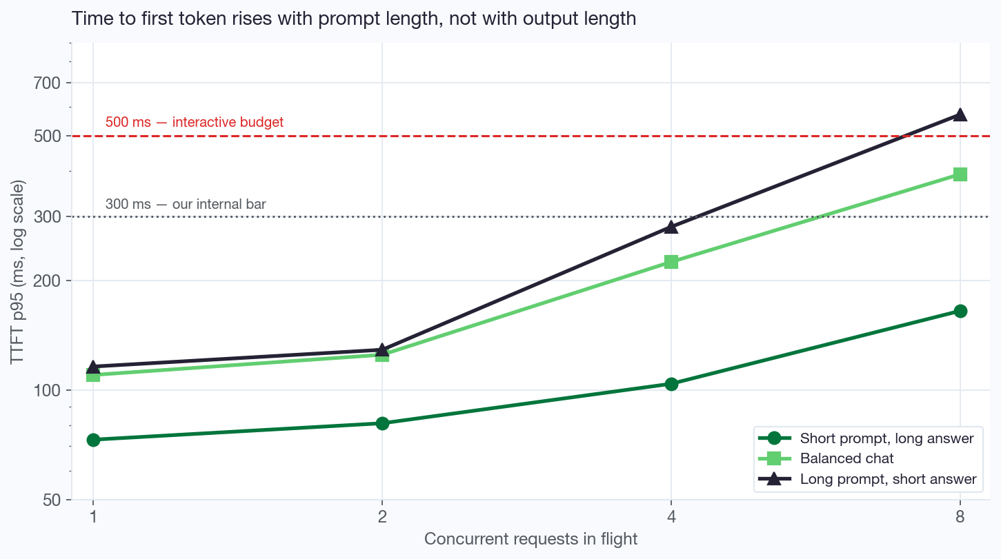
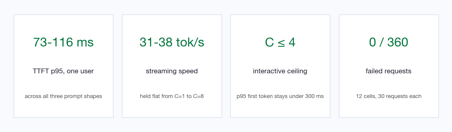
Alone on the machine, this configuration starts fast: p95 first token lands between 73 ms and 116 ms depending on prompt shape. That is well inside anything a person perceives as instant.

Then the three lines fan apart, and they fan apart in the order the mechanism predicts. Short prompts barely notice concurrency — 73 ms at C=1, still only 165 ms at C=8, because there is very little prefill work to contend over. Long prompts degrade first and fastest — comfortable at 116 ms alone, 281 ms at C=4, and 572 ms at C=8, roughly five times the single-user figure. Balanced chat sits between the two throughout, which is what a mixed prompt distribution should do.

Nothing here is a defect. It is prefill contention, visible in a chart: concurrent long prompts queue behind one another for the same arithmetic units, and the queue is what you are looking at. The practical reading is that your prompt shape decides your concurrency ceiling, and a single headline TTFT number for a SKU is close to useless without it.

The tail is where the truth is

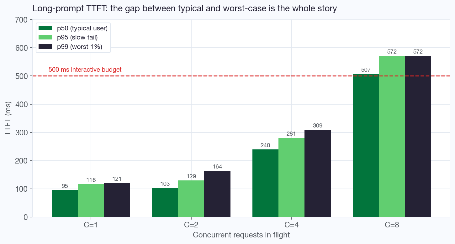
This is the chart that justifies carrying three percentiles instead of one.

At C=1 the bars are almost the same height — 95 ms, 116 ms, 121 ms. With no queue, TTFT is pure prefill, and prefill on a given prompt is a nearly deterministic amount of arithmetic. A 26 ms spread between the typical user and the worst one in a hundred is the signature of an idle engine.

By C=4 the spread has grown to 69 ms and the median itself has more than doubled, to 240 ms. By C=8 the median is 507 ms — it has crossed the interactive budget on its own — and p95 and p99 have converged at 572 ms, which is what saturation looks like: every request is now waiting for the same queue, so the unlucky ones stop being distinguishable from the typical ones.

That convergence is worth pausing on, because it is counter-intuitive. A widening gap between p50 and p99 means some requests are queueing. A gap that closes again at a high value means all of them are. The first is a capacity warning. The second is a capacity limit.

Streaming speed: remarkably flat

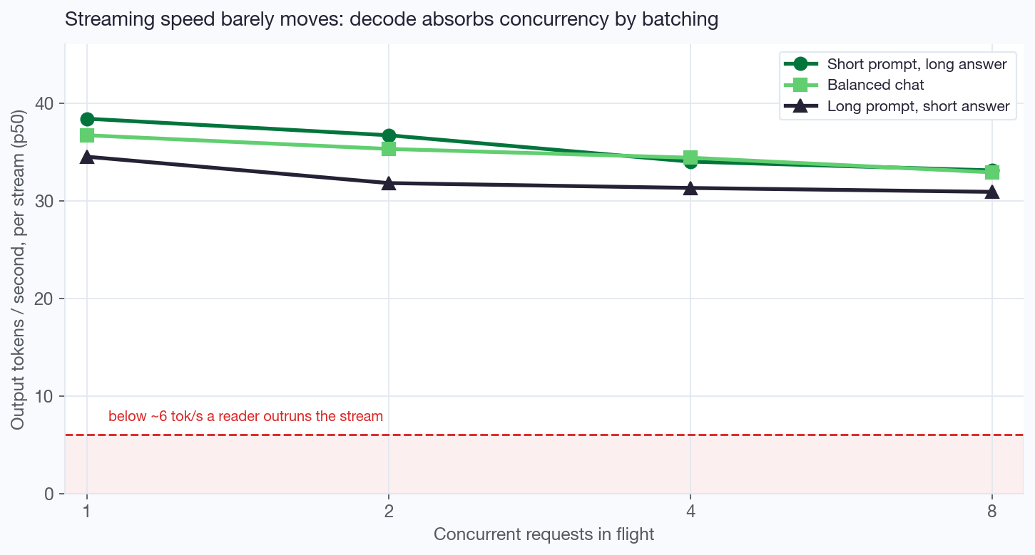
Where TTFT rose five-fold, generation speed holds inside a narrow 31–38 tokens per second band across every cell we ran. Going from one request in flight to eight costs a single stream about four tokens per second — from 38.4 to 33.1 on the decode-heavy bucket, from 34.5 to 30.9 on the prefill-heavy one.

This is decode behaving exactly as a bandwidth-bound workload should. Reading the model’s weights out of memory is the expensive step, and once you have paid for that read you can apply it to eight sequences almost as cheaply as to one. Batching is close to free on this phase, which is the entire reason continuous batching exists as a technique.

Two practical consequences. First, concurrency stretches the wait, not the stream — if a deployment feels slow under load, first-token latency is where to look, not tokens per second. Second, the per-stream figure understates what the machine is doing. At C=8 on the decode-heavy bucket, eight streams at ~33 tok/s each means the node is producing roughly 310 tokens per second in aggregate, and that is the number that matters for anything running offline.

End to end: set by how much you asked for

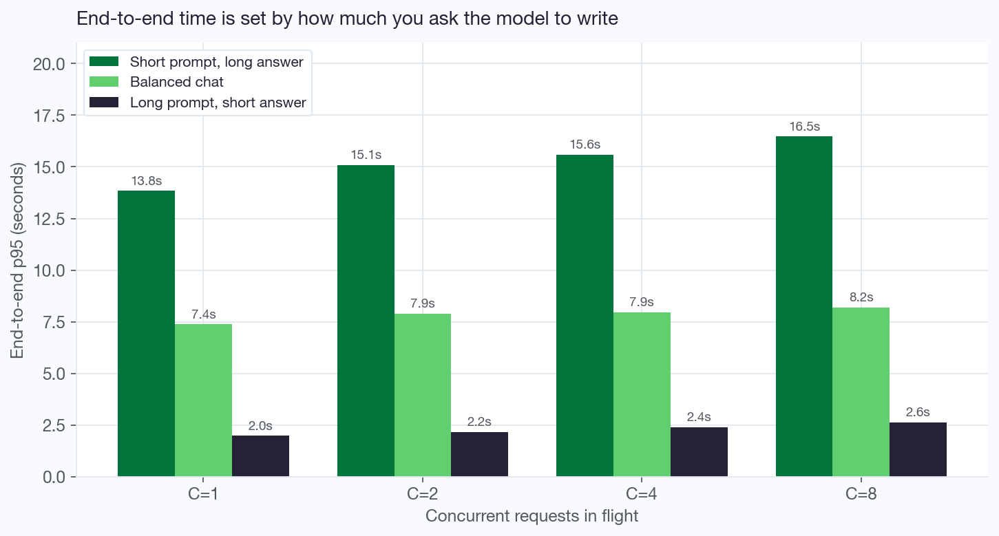
This chart is a useful corrective to the first one. Ranked by end-to-end time, the ordering reverses: the bucket with the best TTFT has the worst E2E, by a factor of seven.

A long prompt with a short answer completes in about 2.0 seconds at p95 and only stretches to 2.6 s at C=8. A short prompt with a long answer takes 13.8 seconds alone and 16.5 s at C=8. The concurrency effect is real but small — a 19% increase from C=1 to C=8 — while the effect of asking for 512 tokens instead of 64 is a factor of seven.

Which is simply E2E ≈ TTFT + output tokens × TPOT made visible. At ~30 ms per token, every 100 tokens you ask for costs three seconds, and no hardware decision changes that as much as an instruction to be concise does. If your users complain about total time, the highest-leverage fix is usually max_tokens, not a bigger GPU.

Nothing failed, at any concurrency

Zero failures in all twelve cells. 360 measured requests, 0% error rate everywhere, including the saturated ones. Under sustained load the engine degraded in latency and never in correctness — which is the behaviour you want, and is consistent with the KV cache never having been exhausted. An engine that starts returning errors under load is a different and much worse problem than one that simply gets slower.

What the gateway hop costs

Everything above bypasses the API gateway. In production nothing does — requests arrive through LiteLLM, which handles authentication, model routing, key-scoped access and usage accounting. That layer is not free, and publishing engine numbers while quietly serving customers through a proxy would be dishonest, so we measured it.

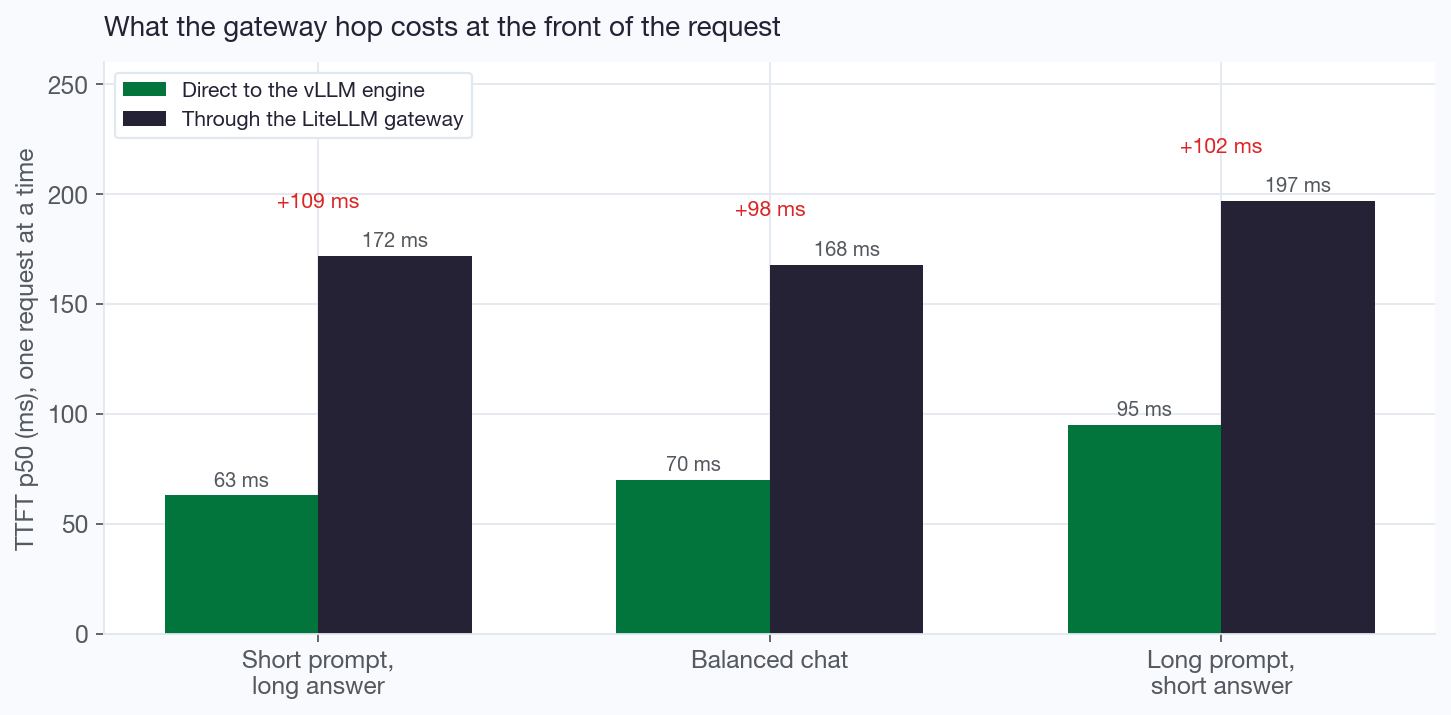
The gateway adds roughly 100 ms to first-token latency and essentially nothing to everything after it. Through LiteLLM, median TTFT lands at 168–197 ms against 63–95 ms direct, while TPOT holds at 26–28 ms per token and decode throughput stays at 36–38 tok/s — the same band the engine produces on its own.

That shape makes sense. The gateway does its work once, at admission: parse the request, authenticate the key, check the key is allowed this model, pick a backend, open the upstream connection. Then it becomes a pipe, and streamed tokens flow through a pipe at the speed the engine produces them. A proxy taxes the front of the request, not the body of it.

Two caveats, because this is a comparison across two runs rather than a controlled experiment. The gateway measurements were taken with synthetic padded prompts of roughly 1,019, 558 and 127 input tokens rather than ShareGPT traces, and they are medians at a single request in flight. Read the ~100 ms as a well-supported order of magnitude, not a calibrated constant. It is enough to plan with: if your first-token budget is 500 ms, roughly a fifth of it belongs to the gateway before the model has done anything at all.

Against what the industry expects

A number means nothing without a threshold beside it. These are the published ones, and where this deployment lands against each — measured at p95, because that is the percentile an SLO is written against.

Published expectation	Source	This deployment (p95)
Interactive chat: TTFT under 500 ms	LLM Inference Handbook	Met for every prompt shape through C=4; at C=8 met for short and balanced, missed for long prompts (572 ms)
Strict goodput SLO: 95% of chats under 200 ms	LLM Inference Handbook	Met for short prompts at every concurrency, and for all shapes at C≤2
Inline code completion: TTFT under 100 ms	LLM Inference Handbook	Only short prompts at C≤2. Not a code-completion SKU
Coding agents: TTFT under 1 s is acceptable	Together AI	Met everywhere, including the worst cell we ran
Interactive coding: 60–90 tok/s typical, 400+ fast	Infercom	31–38 tok/s — below the comfortable band for agentic coding
Comfortable reading: roughly 6 tok/s	Reading-speed convention	Cleared by more than 5× in every cell

Read together those rows draw a clear and quite defensible line. On first-token latency this configuration is genuinely competitive — it clears the standard interactive budget with room to spare, and at low concurrency it clears the strict one. On sustained generation speed it is mid-tier: entirely fine for a human reading prose, well short of what an agent chewing through hundreds of thousands of tokens wants. The age of the cards shows in bandwidth, not in responsiveness.

What to do with these numbers

A benchmark that does not end in a provisioning decision was a waste of GPU hours. So, concretely.

Where to set concurrency

Question	Answer from this run
How good is it for one user?	TTFT p95 73–116 ms, 34–38 tok/s, zero errors. Comfortably instant
Interactive ceiling across all prompt shapes?	C=4. Even long-prompt p95 stays at 281 ms — inside our 300 ms internal bar
Ceiling for short prompts and batch work?	C=8 and beyond. p95 stays ≤165 ms on short→long, with no errors
Where does it actually hurt?	Long prompts at C=8 — p95 TTFT 572 ms, roughly 5× the single-user figure
What is the failure mode?	Slower, never wrong. 0% errors in all twelve cells

Which workloads this fits

Interactive chat and assistants — run it at C≤4. This is the core case and the configuration handles it well. First-token latency stays inside the interactive budget for every prompt shape we tested, streaming runs at 34 tok/s, and an internal assistant, documentation Q&A bot or support-drafting tool for a team of a few dozen people will rarely exceed four requests in flight. One replica covers it.

Retrieval-augmented answering — run it at C≤4, and watch your context length. RAG is the long-prompt bucket, and it is the shape that degrades first. Keep concurrency at four or below, or shorten the retrieved context. This is also the workload with the most headroom left on the table: turning prefix caching back on, which we disabled for measurement honesty, directly attacks the cost of a shared system prompt.

Batch and offline work — run it at C=8 and stop worrying about TTFT. Classification, entity extraction, summarisation, metadata enrichment, synthetic data generation, nightly report drafting. Nobody is watching, so first-token latency is irrelevant and only aggregate throughput counts. At roughly 310 tokens per second sustained, a single node produces on the order of 26 million tokens per day. For a batch pipeline that is serious volume from hardware several generations old, and it is where these cards genuinely earn their keep.

Not inline code completion, and not real-time voice. Both budget first-token latency at or below 100 ms, and both need that budget met at the tail rather than the median. Only our shortest prompts get there, and only when the engine is nearly idle. This is a hardware and model-size question, not a tuning question — no flag in the config above will fix it, and we would rather say so than sell it.

Careful with agentic workloads. An agent chaining ten model calls pays end-to-end latency ten times over, not TTFT. On the balanced bucket at C=4 that is roughly 80 seconds of pure inference for ten steps — workable for a background agent that reports when it is done, frustrating for one a person is watching. And for interactive software development, the comfortable band starts near 400 tokens per second per stream, an order of magnitude above what these cards deliver.

Three rules for sizing from this

1. Size by prompt shape, not by headline number. The three prompt shapes differ by up to 3.5× in first-token latency and 7× in end-to-end time. Find the shape that matches your traffic before you trust any figure here.
2. Size by requests in flight, not by user count. Fifty people using an assistant is not concurrency 50. Measure what is actually in flight at peak, and you will usually find it is a single-digit number.
3. Budget the gateway. Add roughly 100 ms to every TTFT figure here before comparing it to your own SLO, because your users will reach the model through a proxy even though this benchmark did not.

The bottom line: a strong interactive 7B lane on V100s, provided concurrency stays honest, and a genuinely good batch engine above that. It is not a “hundreds of concurrent users on one replica” story, and we would rather state that plainly than sell a fantasy that falls over in week two.

What this post is not

• Not a gateway benchmark. The main measurements go straight to the engine. The gateway is measured separately, on a different prompt corpus, at p50 only.
• Not a saturation study. We stopped at C=8. The knee for long prompts is clearly below that; where the engine actually falls over is a separate run.
• Not a cross-hardware bake-off. The V100/A100/H100 table is published specifications, not our measurements. Choose by rate and euros per million tokens for your workload.
• Not every model size. 7B at TP=4 on this node only. A 14B model on the same four cards behaves differently enough that none of these figures transfer.
• Not fully tuned. Prefix caching and CUDA graphs are both disabled. Both would improve the results; both were disabled deliberately so the numbers describe the hardware rather than a cache-hit rate.
• Not a quality evaluation. Every number here is about speed. Whether the answers are correct, safe and unbiased is measured with entirely different instruments, and it matters more than any of this.

What we measure next

1. Push past C=8 on the long-prompt bucket until something breaks, and publish where the knee actually is rather than where we stopped looking.
2. Prefix caching on, to quantify how much of the RAG-shaped TTFT penalty a shared system prompt gives back.
3. CUDA graphs on, now that Volta boot behaviour is understood, to claim the decode headroom we are currently leaving unclaimed.
4. A controlled gateway A/B on identical ShareGPT prompts, so the ~100 ms figure becomes a measurement instead of an estimate.
5. Record input token counts and persist raw per-request data off the Job volume, so the next post derives nothing at all.

We will publish those as they land, including the ones that make the hardware look worse.